Regression Assumptions: What Researchers Should Check
A regression’s results are only trustworthy if its assumptions hold—yet those assumptions are the most commonly skipped step in applied work. This is a practical checklist: what each assumption is, how to check it, and what to do when it fails.
Running a regression is easy; running one you can defend is not. The gap between the two is almost entirely a matter of assumptions—the conditions that must hold for the coefficients, standard errors, and p-values to mean what they appear to mean. Software will estimate a regression on any data you give it and report tidy, significant-looking results whether or not those conditions are met. Checking the assumptions is the step that separates a credible analysis from a plausible-looking one, and it is the step reviewers scrutinise first.
This guide is a practical, plain-language checklist of the assumptions behind ordinary regression: what each one is, how to check it, and how to respond when it fails. It is the companion to our overview of OLS regression, which explains why these assumptions matter; here the focus is entirely on the doing. It reflects the diagnostic discipline in our Econometrics & Quantitative Research practice.
Start with the residuals
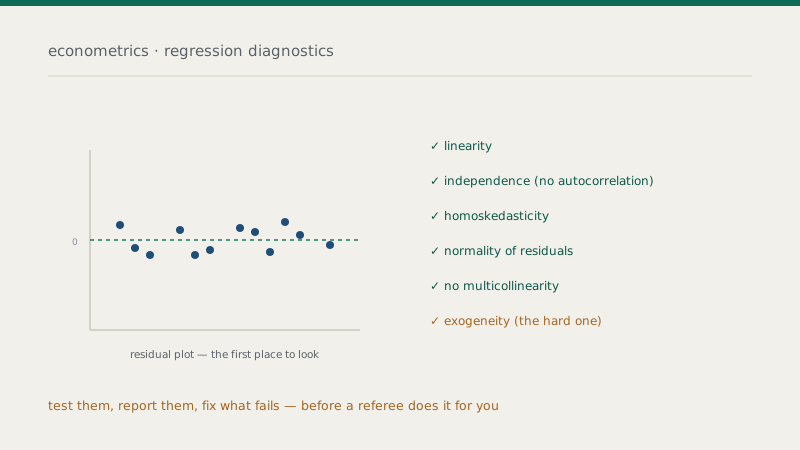
Before the individual assumptions, one habit underlies most diagnostics: look at the residuals. The residuals—the differences between observed and predicted values—carry the evidence for or against most of the assumptions, because the assumptions are largely about the behaviour of the errors, which the residuals estimate. A handful of residual plots (residuals against fitted values, against each predictor, and a plot of their distribution) reveals non-linearity, non-constant variance, and outliers at a glance. Plotting the residuals is the single most informative diagnostic step, and it comes before any formal test.
Linearity
What it assumes: the relationship between the predictors and the outcome is linear in the parameters. How to check: plot residuals against fitted values and against each predictor—a clear curve or pattern signals non-linearity. What to do: transform variables (for example, a log transformation), add polynomial or interaction terms, or use a more flexible functional form. Fitting a straight line to a genuinely curved relationship produces biased, misleading coefficients, so this is worth getting right early.
Independence of errors (no autocorrelation)
What it assumes: the errors are not correlated with one another. How to check: this matters most in time-series and panel data, where errors in nearby periods often move together; tests such as Durbin–Watson or Breusch–Godfrey detect it, and plotting residuals over time helps. What to do: use standard errors that account for autocorrelation (such as Newey–West), model the dynamics explicitly, or—in panels—cluster the standard errors. Ignoring autocorrelation leaves the coefficients unbiased but the standard errors wrong, so significance can be badly overstated.
Homoskedasticity (constant error variance)
What it assumes: the spread of the errors is constant across the range of the predictors. How to check: a residuals-versus-fitted plot showing a fan or cone shape is the classic sign; formal tests include Breusch–Pagan and White. What to do: the standard, low-cost remedy is robust (heteroskedasticity-consistent) standard errors, which correct the inference without changing the coefficients—many applied researchers now use them by default. Heteroskedasticity does not bias the coefficients, but it invalidates the usual standard errors, so the fix is about trustworthy inference.
Distinguish two kinds of violation. Some (heteroskedasticity, autocorrelation) corrupt only the standard errors—fixable after estimation with robust or clustered errors. One—endogeneity—biases the coefficients themselves and cannot be patched; it requires a different identification strategy. Knowing which kind you face determines the fix.
Normality of residuals
What it assumes: the residuals are approximately normally distributed. How to check: a histogram or Q–Q plot of the residuals, optionally a formal test such as Shapiro–Wilk. What to do: in reasonably large samples this assumption is the least critical—the central limit theorem means inference is robust to moderate non-normality—so mild departures are rarely a problem. Severe non-normality, or heavy outliers driving it, may call for a transformation or a robust estimation approach. Do not over-worry this one in large samples; do take it seriously in small ones.
No perfect multicollinearity
What it assumes: no predictor is an exact linear combination of the others. How to check: perfect collinearity stops the model from estimating at all; the practical concern is high collinearity, checked with the variance inflation factor (VIF) or a correlation matrix of predictors. What to do: high collinearity inflates standard errors and makes individual coefficients unstable and hard to interpret—though it only matters when you need that individual effect. Consider removing or combining redundant predictors, or accept that some individual effects cannot be separated. Note that it does not bias the coefficients or harm overall prediction; it just clouds the individual estimates.
Exogeneity: the hard one
What it assumes: the predictors are uncorrelated with the error term. How to check: there is no simple plot or single test—assessing it is a matter of reasoning about your data and design (are there plausible omitted confounders? could causality run backwards? is a key variable measured with error?), sometimes supported by specific tests when an instrument is available. What to do: this is the assumption whose failure—endogeneity—is most serious, because it biases the coefficients themselves and blocks any causal reading. The remedies are structural: instrumental variables, panel methods, or a quasi-experimental design. It is the assumption most likely to be quietly violated and most likely to draw a reviewer’s objection, and it cannot be fixed after the fact.
A workflow you can follow
Bringing it together, a disciplined diagnostic routine looks the same every time. Estimate the model, then plot the residuals as a first look. Work through the assumptions relevant to your data type—linearity, independence, homoskedasticity, normality, collinearity—using the appropriate plots and tests. Reason explicitly about exogeneity, since no test substitutes for judgement there. Apply the right remedy for each violation you find: robust or clustered standard errors for variance and correlation problems, transformations for non-linearity, and a genuine identification strategy for endogeneity. Then report what you checked and what you did—a results section that shows its diagnostics is far more convincing than one that hides them.
The underlying point is that assumption checking is not a formality to rush through on the way to the results; it is what makes the results mean anything. A regression whose assumptions have been tested, whose violations have been addressed, and whose diagnostics are reported is a regression a reader can trust. One presented as a bare table of coefficients invites the reviewer to ask all the questions you should have asked yourself—which is exactly the situation a careful researcher avoids.
Frequently asked questions
Want your regression diagnostics done properly?
From residual analysis and formal tests to robust inference and endogeneity strategies, our team can run the full diagnostic suite—and report it the way reviewers expect.