OLS Regression: What Researchers Should Know

Ordinary least squares—OLS—is so common that most researchers run it almost without thinking. Type the command, read the coefficients, report the significant ones. But OLS is not a black box that returns truth; it is a specific estimator that produces trustworthy results only when specific conditions hold. When they don’t, it can return confident, precise-looking numbers that are biased or whose significance is illusory. Understanding what OLS does and what it assumes is the difference between using it and being used by it.

This guide explains what OLS estimates, the assumptions its reliability rests on, and what to do when they fail. It builds on our guide to correlation vs regression and sits within our Econometrics & Quantitative Research practice, where getting these fundamentals right is the starting point for everything else.

What OLS actually does

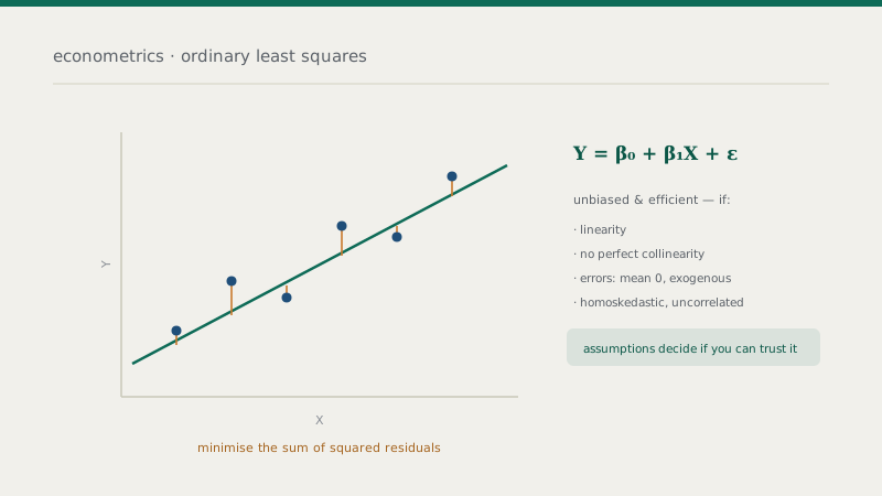
OLS fits a line—or, with several predictors, a plane—through your data by choosing the coefficients that make the model’s predictions as close to the observed values as possible. Specifically, it minimises the sum of squared residuals: the residual is the gap between each observed value and the value the model predicts, and OLS picks the coefficients that make the total of those squared gaps as small as possible. Squaring means larger errors count disproportionately, and it makes the mathematics tractable and the solution unique.

The result is a set of estimated coefficients—an intercept and a slope for each predictor. Each slope has a natural interpretation: it is the average change in the outcome associated with a one-unit change in that predictor, holding the others constant. Alongside the coefficients, OLS produces standard errors that quantify how precisely each is estimated, which in turn drive the t-statistics, p-values, and confidence intervals researchers rely on for inference. That inference, however, is only as trustworthy as the assumptions behind it.

Why OLS is popular: the BLUE property

OLS is not popular merely by habit. Under a set of standard assumptions, it has a genuinely attractive property: it is the Best Linear Unbiased Estimator, often abbreviated BLUE. “Unbiased” means that, on average across repeated samples, it gets the true coefficient right—it doesn’t systematically over- or under-estimate. “Best” means that among all linear unbiased estimators, it has the smallest variance—it is the most precise. This result, which comes from the Gauss–Markov theorem, is why OLS is the default: when its assumptions hold, no other linear unbiased estimator does better.

The crucial words, though, are “when its assumptions hold.” The BLUE property is conditional. Every part of it—unbiasedness, efficiency, and the validity of the standard errors that inference depends on—rests on assumptions about the model and the data. Which is why knowing those assumptions is not academic pedantry; it is what tells you whether your regression output means what you think it means.

The assumptions that matter

OLS reliability rests on a handful of assumptions. You do not need to memorise formal statements, but you do need to understand what each protects against.

Linearity. The relationship between the predictors and the outcome is linear in the parameters. If the true relationship is curved and you fit a straight line, the model is misspecified and the estimates are misleading. (And for a binary outcome, a linear model is the wrong choice entirely—see logistic regression.)

No perfect multicollinearity. No predictor is an exact linear combination of others. Perfect collinearity makes the coefficients impossible to estimate; high-but-imperfect collinearity inflates their standard errors, making effects hard to detect—a common practical problem worth checking.

Exogeneity (zero-conditional-mean errors). The error term has a mean of zero given the predictors—in effect, the predictors are uncorrelated with whatever the model leaves out. This is the most consequential assumption, because its failure is endogeneity, which biases the coefficients and blocks any causal reading. Omitted variables, reverse causality, and measurement error all violate it.

Homoskedasticity. The errors have constant variance across the range of the predictors. When they don’t—heteroskedasticity’s cross-sectional cousin—the coefficients remain unbiased but the standard errors are wrong, so the p-values and confidence intervals cannot be trusted.

No autocorrelation. The errors are uncorrelated with one another. This matters especially in time-series and panel data, where errors in adjacent periods often move together; ignoring it again distorts the standard errors.

Normality of errors is sometimes added, but chiefly matters for exact small-sample inference; in reasonably large samples it is the least critical of the set.

What to do when assumptions fail

The point of knowing the assumptions is to test them and respond, not to abandon OLS at the first violation. Different failures call for different remedies. Heteroskedasticity and autocorrelation, which corrupt the standard errors but not the coefficients, are routinely handled with robust or clustered standard errors that correct the inference without changing the estimates. Non-linearity can be addressed by transforming variables or specifying the functional form more flexibly. High multicollinearity may call for rethinking which variables belong in the model.

Endogeneity is the serious one, because it biases the coefficients themselves—and no robust standard error fixes bias. Addressing it requires a different strategy: instrumental variables, panel methods such as fixed effects, or a quasi-experimental design. This is why endogeneity is treated at length on its own: it is the assumption whose failure most often turns a regression into a misleading one, and it cannot be patched after the fact.

The disciplined workflow is therefore always the same: run the regression, then run the diagnostic tests appropriate to your data, address any violations with the right remedy, and report what you found and did. A regression presented with its assumptions tested and its diagnostics shown is credible; the same regression presented as a bare table of significant coefficients invites exactly the objections a careful reviewer raises first.

The bottom line

OLS is powerful, interpretable, and—under its assumptions—provably the best linear unbiased estimator, which is why it remains the foundation of empirical research. But it is powerful only conditionally. It will always return coefficients and p-values; whether those numbers mean anything depends on assumptions the software will never check for you. Treat OLS not as a button that produces answers but as an estimator whose output you are responsible for validating, and it becomes exactly what it should be: a reliable, transparent tool for understanding your data.