Making Time Series Stationary (and Why It Matters)

Time-series data—a variable observed at regular intervals over time—has a property that makes it both powerful and treacherous: successive observations are related to one another. That structure is what lets us forecast, but it also means the standard assumptions behind ordinary regression often do not hold. At the centre of this sits a single concept that trips up more time-series analyses than any other: stationarity. Get it wrong and you can produce a highly significant relationship between two variables that have nothing to do with each other.

This guide explains what stationarity means, why it is so consequential, how to test for it, and what to do when your series is non-stationary—including the important case where non-stationary series can legitimately be analysed together. It reflects how we handle time-series work in our Forecasting & Predictive Analytics practice.

What stationarity means

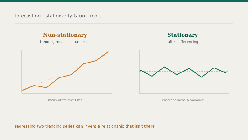
A time series is stationary if its statistical properties do not change over time—most importantly, its mean and variance are constant, and the relationship between observations depends only on the distance between them, not on when they occur. A stationary series fluctuates around a stable level; it has no trend and no systematic change in volatility. A non-stationary series, by contrast, has properties that drift: a trending mean, a changing variance, or both.

The reason this matters is that most classical time-series methods—and the statistical theory that makes their inference valid—assume stationarity. When you apply those methods to non-stationary data, the standard errors, test statistics, and significance levels they produce are simply not trustworthy. The tools are working correctly; they are just being fed data that violates their assumptions, and the output is misleading.

The spurious regression problem

The clearest illustration of why this matters is spurious regression. Take two completely unrelated variables that both happen to trend upward over time—each rising for its own reasons. Regress one on the other, and you will very often find a large, highly significant coefficient and an impressive fit. It is an illusion. The regression is not detecting a relationship between the variables; it is detecting that both are trending, and mistaking shared movement over time for a genuine connection.

This is not a rare edge case. It is a systematic trap that has produced countless meaningless “findings,” and it is exactly the kind of error a knowledgeable reviewer looks for first in a time-series paper. Two trending series will appear related far more often than chance would suggest, and the apparent significance is worthless. Establishing stationarity—or handling non-stationarity correctly—is what protects you from reporting a relationship that does not exist.

Testing for stationarity

You should never simply assume stationarity—or non-stationarity—from a plot alone, though plotting the series is always a sensible first look. The formal tools are unit-root tests, which assess whether a series contains a “unit root,” the technical signature of a particular and common kind of non-stationarity. The most widely used is the Augmented Dickey–Fuller test; others, such as the Phillips–Perron and KPSS tests, approach the question from complementary angles.

A subtlety worth knowing is that these tests frame the question differently. The Augmented Dickey–Fuller and Phillips–Perron tests take non-stationarity as the starting hypothesis, so failing to reject it is not the same as confirming stationarity. The KPSS test reverses this, taking stationarity as the null. Because they are set up differently, using them together gives a more robust picture than relying on any single test—a practice careful analysts follow and reviewers appreciate.

How to make a series stationary

When a series is non-stationary, the usual remedy is differencing: instead of analysing the level of the variable, you analyse the change from one period to the next. Differencing removes a trend of the kind associated with a unit root, and a series that becomes stationary after being differenced once is called integrated of order one. Occasionally a series must be differenced twice, but needing more than that is unusual and often a sign something else is going on.

Differencing is not the only tool. A series whose variance grows over time can sometimes be stabilised with a transformation such as taking logarithms before differencing. A series that is stationary around a deterministic trend—rather than containing a unit root—may be handled by including a trend term instead of differencing. Distinguishing these cases matters, because differencing a trend-stationary series, or detrending a unit-root series, can each introduce their own problems. The right treatment depends on the kind of non-stationarity you actually have, which is why testing comes first.

When non-stationary series belong together: cointegration

Here is where it becomes genuinely interesting. Differencing solves the stationarity problem, but it also throws information away: by analysing only changes, you lose the long-run relationship between the levels of the variables. Sometimes that long-run relationship is exactly what you care about—and sometimes two non-stationary series are tied together in the long run even though each wanders on its own.

This is the idea of cointegration: two or more non-stationary series can share a stable long-run equilibrium relationship, such that a particular combination of them is stationary even though each series individually is not. When variables are cointegrated, simply differencing them all and running a standard model discards the very relationship of interest. Instead, models built for cointegrated data—error-correction models and related approaches—let you capture both the short-run dynamics and the long-run equilibrium. Recognising cointegration is what separates a naive “difference everything” approach from an analysis that respects the real structure of the data, and it is a common expectation in applied macroeconomic and financial work.

The bottom line

Stationarity is not a technicality to wave through on the way to a result—it is the assumption that determines whether your time-series inference means anything at all. Non-stationary data invites spurious regression, where trending variables appear related but are not. So test for stationarity using unit-root tests, ideally more than one; make series stationary by the method that matches the kind of non-stationarity you have, usually differencing; and check for cointegration before differencing away a long-run relationship you may want to study. Handle stationarity properly and your time-series results are trustworthy. Ignore it, and the most impressive coefficient in your table may be pure illusion.