Difference-in-Differences Explained

Suppose a region introduces a policy—a minimum-wage increase, a new regulation, a training programme—and you want to know its effect. You cannot run a randomised experiment; the policy simply happened. You could compare outcomes in the region before and after, but other things changed over that period too, so any difference might have nothing to do with the policy. You could compare the treated region to an untreated one after the policy, but the two regions may have differed all along. Each simple comparison is confounded. Difference-in-differences is the elegant idea that combines them to cancel out much of the confounding.

It has become a workhorse of applied economics, management, and policy evaluation precisely because it turns naturally occurring events into credible evidence. This guide explains the logic, the all-important parallel-trends assumption, and—critically—the recent methodological developments that have changed how the method should be applied. It sits within our Causal Inference & Policy Evaluation practice and builds on our guide to endogeneity, the problem DiD is designed to overcome.

The core idea

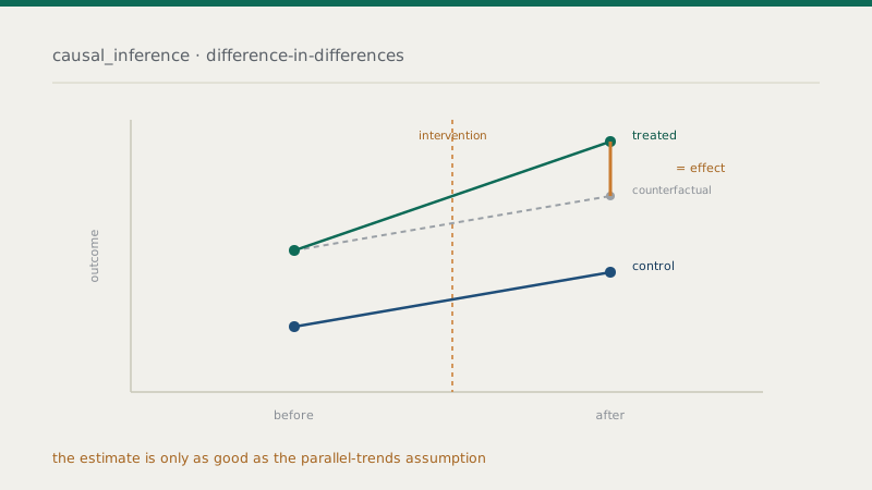
Difference-in-differences compares the change in an outcome for a group affected by an intervention (the treated group) with the change over the same period for a group that was not affected (the control group). The first “difference” is before-versus-after within each group; the second “difference” is treated-versus-control. Taking the difference of these differences isolates the effect of the treatment.

The reason this works is that each comparison cancels a different source of bias. Comparing before and after within the treated group removes anything about that group that stayed constant—but it leaves in any general trend over time affecting everyone. Subtracting the control group's change over the same period removes that common trend, because the control group experienced it too but not the treatment. What remains—the difference in the differences—is the treatment effect, provided one key condition holds.

The parallel-trends assumption

The entire method rests on a single, crucial assumption: parallel trends. It states that, in the absence of the treatment, the treated and control groups would have followed the same trend over time. The control group's change is used as a stand-in for what would have happened to the treated group had the treatment never occurred—the counterfactual. If the two groups would have moved in parallel anyway, the control group's trend is a valid counterfactual, and the extra movement in the treated group is the effect. If they would not have moved in parallel—if the treated group was already on a different trajectory—then difference-in-differences attributes that pre-existing divergence to the treatment, and the estimate is biased.

Parallel trends is an assumption about a counterfactual, so it can never be proven directly—we cannot observe what would have happened. But its plausibility can be assessed. The most common check is to examine whether the groups moved in parallel before the treatment: if several pre-treatment periods show the treated and control groups trending together, the assumption is more credible for the post-treatment period. This is why researchers plot pre-trends and why reviewers expect to see them. A visible divergence before treatment is a serious warning sign.

What can go wrong

Beyond a failure of parallel trends, several issues can undermine a difference-in-differences design. One is anticipation: if the treated group changes its behaviour before the treatment formally begins—because the policy was announced in advance, say—the pre-period is contaminated. Another is spillovers: if the treatment affects the control group indirectly, the control group is no longer a clean counterfactual. A third is compositional change: if the make-up of the groups shifts over the study period, before-and-after comparisons within a group are no longer comparing like with like. Each of these is a threat to be argued against, not assumed away.

The staggered-adoption revolution

The most important recent development concerns what happens when different units are treated at different times—so-called staggered adoption, extremely common in policy research where jurisdictions adopt a policy in different years. For a long time, the standard way to handle this was a two-way fixed-effects regression, and it was applied almost automatically.

A wave of methodological research has since shown that the two-way fixed-effects estimator can be badly biased under staggered adoption, particularly when treatment effects change over time. The technical reason is that the estimator implicitly uses already-treated units as controls for later-treated ones, which can contaminate the comparison and, in some cases, even produce an estimate with the wrong sign. This is now widely understood in the field, and a range of newer estimators has been developed to handle staggered designs correctly. The practical implication is significant: a staggered difference-in-differences analysis that relies on the old two-way fixed-effects approach is increasingly likely to draw a reviewer's objection, and current best practice is to use one of the newer robust estimators and to report the results transparently. Knowing this is now part of applying the method competently.

When difference-in-differences is a good fit

Difference-in-differences is well suited to situations where an intervention affected some units and not others, where you have outcome data both before and after for both groups, and where you can make a credible case for parallel trends. It is a natural tool for evaluating policies, regulations, programmes, and other discrete events that create a treated and an untreated group. It is less suitable when no comparable control group exists, when the treatment was adopted precisely because the treated group was already on a different trajectory, or when only post-treatment data is available.

Where a clean control group is hard to find, related designs may serve better: a regression-discontinuity design when treatment is assigned by a threshold, or a synthetic-control approach when a single treated unit can be compared to a weighted combination of untreated ones. Choosing among these is part of designing a credible evaluation, and it depends—as always—on the setting and the data.

The bottom line

Difference-in-differences earns its popularity: it converts naturally occurring events into credible causal evidence by differencing away both fixed group differences and common time trends. But its credibility lives or dies on the parallel-trends assumption, which must be argued and supported with pre-trend evidence rather than assumed. And for the common case of staggered adoption, the method has genuinely moved on—the old two-way fixed-effects default can mislead, and modern robust estimators are now expected. Used with those cautions in mind, difference-in-differences remains one of the most powerful and defensible tools in the applied researcher's kit.