How to Evaluate a Forecast: Accuracy Metrics and Out-of-Sample Testing

Building a forecasting model is the easy part; knowing whether it is any good is where most forecasting work goes wrong. The temptation is to judge a model by how well it fits the historical data it was built on—but that number says almost nothing about how it will perform on the future, which is the only thing a forecast is for. Evaluating a forecast properly means testing it on data it has never seen, measuring its errors with the right metrics, and—crucially—checking that it beats a simple benchmark. Skip any of these, and an impressive-looking model can be worthless.

This guide covers the accuracy metrics, the out-of-sample testing that gives them meaning, and the benchmark comparison that keeps forecasters honest. It complements our guide to making time series stationary and reflects the evaluation-first approach in our Forecasting & Predictive Analytics practice.

Why in-sample fit is not enough

The most common and costly forecasting error is judging a model by its fit to the data it was estimated on—its in-sample performance. A sufficiently flexible model can fit historical data almost perfectly and still forecast terribly, because a close fit to the past can reflect overfitting—the model has learned the noise in the historical sample rather than the genuine pattern. An impressive in-sample fit is therefore not evidence of a good forecast; if anything, a near-perfect one is a warning sign.

What matters is out-of-sample performance: how accurately the model predicts data it did not use during estimation. This is the whole point of forecasting—predicting the unknown—so it is the only test that reflects the task. Any evaluation that reports only in-sample fit has not actually tested the forecast at all.

Out-of-sample testing

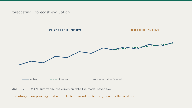
The foundational method is to split the data by time. You hold back the most recent portion as a test set, estimate the model on the earlier training set, then generate forecasts for the test period and compare them to what actually happened. Because the model never saw the test data during estimation, its accuracy there is an honest estimate of how it will perform going forward. The temporal order matters: unlike cross-sectional data, time-series data must be split chronologically—training on the past and testing on the future—since using future data to predict the past leaks information and inflates apparent accuracy.

A more robust approach is time-series cross-validation (rolling or expanding windows), which repeats the exercise across multiple successive cut-off points—forecasting the next period, rolling the window forward, and forecasting again—then averages the results. This uses the data more fully and gives a more stable picture of accuracy across different periods, rather than resting the whole verdict on one arbitrary split. Whichever you use, the principle is inviolable: never evaluate a forecast on data the model was trained on.

Accuracy metrics

Once you have out-of-sample forecasts and the actual values, you measure the errors—the differences between them—and summarise with an accuracy metric. Several are standard, and each has a character worth knowing.

Mean absolute error (MAE) is the average size of the errors, in the original units. It is intuitive and treats all errors proportionally. Root mean squared error (RMSE) is also in the original units but squares the errors before averaging, so it penalises large errors more heavily—useful when big misses are especially costly, but more sensitive to outliers. Mean absolute percentage error (MAPE) expresses errors as a percentage of the actual values, which makes it scale-independent and easy to communicate—but it breaks down when actual values are near zero and penalises over- and under-forecasting asymmetrically, so it must be used with care.

No single metric is universally best. MAE and RMSE are in the data’s units and so can’t be compared across different series; MAPE is comparable across series but has known pathologies. The sensible practice is to report more than one, choose the metric that matches what actually matters for your problem (are large errors disproportionately bad? do you need scale-independence?), and be explicit about which you used and why.

The benchmark test

Here is the step that separates serious forecast evaluation from the rest, and the one most often skipped: compare your model against a simple benchmark. An accuracy number in isolation—“RMSE of 4.2”—is meaningless, because there is nothing to judge it against. The benchmark provides the yardstick.

The classic benchmark is the naive forecast: for many series, simply predicting that the next value equals the last observed value (or, for seasonal data, the value from the same period last cycle). It sounds trivial, and that is exactly the point—a sophisticated model that cannot beat the naive forecast has added nothing, and a surprising number of complex models fail this test. Establishing that your model beats a sensible naive benchmark, out-of-sample, is the real evidence that it has genuine forecasting value. A forecasting study that does not report this comparison has not made its case, and reviewers increasingly expect to see it.

Putting it together

A credible forecast evaluation follows the same shape every time. Split the data chronologically, or use rolling-window time-series cross-validation. Generate forecasts for the held-out period and compute the errors. Summarise them with appropriate metrics—more than one, chosen to match the problem. And compare the result against a simple benchmark such as the naive forecast, out-of-sample, to show the model earns its complexity. Report all of it transparently, so a reader can see not just that the model is accurate, but that its accuracy was measured honestly and means something.

The underlying discipline is the same one that runs through all predictive work: performance on data the model has already seen proves nothing; performance on data it hasn’t is everything. A forecast evaluated this way can be trusted and defended. One judged on its fit to history is a confident-looking claim about the future built on no real evidence at all.